Atmospheric drag
Part III: Simplified Modeling of Supersonic and High-altitude Effects
This page originally compiled Mar 2007 by TFR
Earth's atmosphere is far from uniform if we are considering flight through it from ground level to orbit. There are many highly accurate models of the atmosphere available if one is so inclined. Here we are mainly concerned with a simple representation of the effects on the motion of our rocket as it travels through a standard atmosphere, "... a hypothetical vertical distribution of atmospheric temperature, pressure and density which, by international agreement, is roughly representative of year-round, midlatitude conditions ..." The standard atmosphere is established by measurement and theory over a period of years by various concerned agencies and institutions. Such a generalized, averaged atmosphere is exactly what we need for our simple models.
Examining our drag equation,
Fd = 1/2ρv2ACd,
only the variable ρ, the density of the air, need be accounted for to model the thinning of the atmosphere with altitude. Density drops not quite exponentially as altitude increases, but for our purposes a simple exponential equation will be sufficient to about ±35%, from about 0 to 100 km altitude:
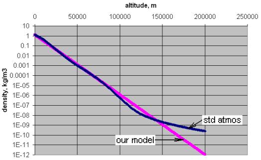 ρ ≈ 1.28e-0.000139h, where:
ρ is the density in kg/m3
e is the base of the natural logarithms, approximately 2.71828
h is the height above sea level, in meters
Above 100 km, where the density has diminished to one millionth or less of that at sea level, we will neglect the effects of atmosphere entirely. For precise applications this would not be appropriate. Orbits of Earth satellites below about 500 km altitude are routinely corrected for atmospheric drag, which changes the orbit slightly with each pass. Where our intent is mainly to simulate the drag on our rocket during launch, we will refer the analysis of orbital drag to the references in the bibliography, some of which develop it in considerable mathematical detail.
Air, being compressible, does not react uniformly to objects traveling through it both slowly and extremely rapidly. It is well known that as the object approaches the speed of sound, known as Mach 1, shock waves begin to form around it, considerably increasing the drag on it. Accurate modeling of this is complex, involving the shape and smoothness of the object and the temperature and humidity of the air, as well as the velocity of the object. In the case of our rocket, the extinguishing of the exhaust gases expelled from the rear would cause increased drag, as the shape presented to the air changed from an extremely long cylinder (the rocket plus its exhaust plume) to a short, bluntly truncated cylinder. For our purposes we can apply a simple variation in Cd to approximate the variation in drag around Mach 1:
 Cd ≈ Cd0300-(1.1-M)2 + 0.01M + Cd0, where:
Cd is the Cd at this Mach number
Cd0 is the Cd at subsonic velocities
M is the Mach number at current velocity
This equation simply doubles Cd at Mach 1.1, and applies a bit of slope (0.01M). One can adjust the variables to suit, if desired: 300 adjusts the width of the peak, 1.1 adjusts the Mach number of the peak, and 0.01 adjusts the slope of the entire curve. As is, it approximates reasonably well for semi-streamlined shapes like rockets.
In order to apply the above variation in Cd, we must know at what Mach number our object is traveling. The speed of sound varies, being mostly dependent on the temperature of the air. Temperature, in turn, is a somewhat complex function of altitude, and varies considerably with weather, etc. For our purposes Mach 1 can be modeled directly, from 0 to 100 km altitude, to about ±3%, with:
M ≈ 2.340×10⁻¹⁷h4 - 4.897×10⁻¹²h3 + 3.227×10⁻⁷h2 - 7.276×10⁻³h + 346.2, where:
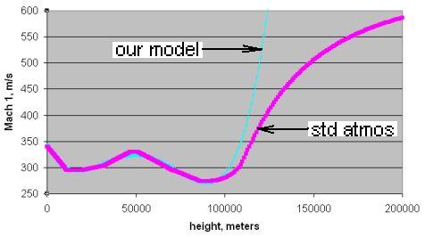 M is Mach 1 at this altitude, in meters/second
h is height above sea level, in meters
We will again ignore these effects above 100 km altitude. Note that our polynomial model is not applicable above 100 km altitude, and will give useless results if used there! The US Standard Atmosphere specifies the speed of sound only up to 86 km altitude, because attenuation of the sound in the ever-thinner air causes the concept to lose its applicability at high altitude, so our approximation has some validity. Note that from 0 to 100 km, Mach 1 does not vary more than ±12% from its mean value, 304.6 m/s, and for our simplified calculations we could just as well use that value as to go to the trouble of applying the polynomial model.
Examples:
An object with Cd of 0.25, a cross-sectional area of 0.1 m2, at 25000 meters altitude, is moving through the air at 300 meters/second. Assuming standard atmosphere:
At what Mach number is it moving?
M ≈ 2.340×10-17250004 - 4.897×10-12250003 + 3.227×10-7250002 - 7.276×10-325000 + 346.2
= 9.141 - 76.516 + 201.688 - 181.9 + 346.2 = 298.6
Mach number = v/M = 300/298.6 = 1.005, the object is barely supersonic
How does this affect its Cd?
Cd ≈ 0.25×300-(1.1-1.005)2 + 0.01×1.005 + 0.25 = 0.2374 + 0.01005 + 0.25 = 0.497, drag is up considerably near Mach 1
What is the air density at this height?
ρ ≈ 1.28×2.71828-0.000139×25000 = 0.0396 kg/m3
What is the resulting drag force on the object?
Fd = 1/2×0.0396×3002×0.1×0.497 = 88.6 kg-m/s2
Finally, if we use the average value for Mach 1, 304.6 m/s, how will our results change?
Mach number = 0.985; Cd = 0.492; Fd = 87.7 kg-m/s2
Home
Last Revised: Apr 2007