Let us again calculate the example from "Projectile at an Angle; Part I":
A projectile is fired at an elevation angle of 30° and an initial velocity of 1000 feet/second. Including atmospheric drag,
What are the x and y components of the initial velocity?
1000 ft/s = 304 m/s,
v0x = 304 cos 30° = 304 × 0.8660 = 263.27 m/s
v0y = 304 sin 30° = 304 × 0.5000 = 152.00 m/s; these are not affected by drag
At this point we must build our numerical simulation, as other parameters will be affected by drag. We will simulate in the same manner as "Atmosphere, Part II", starting with the acceleration equation and continuously summing the results to form the velocity and position. We will need some further information to begin: the drag equation is
Fdrag = -1/2CdρAv2
and we shall have to determine values for Cd, ρ and A. Let us choose for our projectile a common rifle bullet: .308 caliber, 150 grain weight. These correspond to 0.00782 m and 0.00972 kg.
Cd, the drag coefficient, depends on the shape of the object, the smoothness of its surface, and the velocity with which it is passing through the air. For our bullet, we will guess Cd at 0.2, based on available lists of common shapes.
ρ, the density of the air, we will take as 1.2 kg/m3, an average low-altitude value.
A, the cross-sectional area, is simply the frontal area of our bullet. πr2 = 3.14159 × 0.003912 = 0.0000481 m2.
We must find acceleration equations for both motions, vertical and horizontal, which take drag into account. The equation we have been using for falling objects,
a = -g(1 - v2/vt2)
does not work properly if our v is already above vt. We must return to the equation of motion,
ma = ΣF; mass × acceleration = sum of all forces
ma = -mg - 1/2CdρAv2; mass × acceleration = sum of weight and drag; solving for a,
a = -g - (CdρAv2) / (2m)
giving us an expression for vertical acceleration which does not depend on vt. We must take care of the sign of the drag term. Since v is squared, its sign is lost, and we must see that it is opposite that of vertical v: if we are falling, drag force is upward, if we are rising, drag force is downward. Similarly for horizontal,
ma = ΣF; mass × acceleration = sum of all forces
ma = 1/2CdρAv2; mass × acceleration = drag only; solving for a,
a = (CdρAv2) / (2m)
We now have acceleration equations in y and x on which to build our simulation. Let us calculate the first 2 seconds as an example:
t = 1
y calculations:
a = -g - (CdρAv0y2) / (2m) = -9.81 - (0.2 × 1.2 × 0.0000481 × 1522) / (2 × 0.00972) = -23.53 m/s2
vinit = v0y = 152 m/s; velocity at the start of this second
vfinal = vinit + a = 128.47 m/s, velocity at the end of this second
vavg = (vinit + vfinal)/2 = 140.24 m/s, average velocity for this second
sy = vavg = 140.24 m, vertical position at the end of this second
x calculations:
a = (CdρAv0x2) / (2m) = (0.2 × 1.2 × 0.0000481 × 2632) / (2 × 0.00972) = -41.16 m/s2
vinit = v0x = 263.27 m/s; velocity at the start of this second
vfinal = vinit + a = 222.11 m/s, velocity at the end of this second
vavg = (vinit + vfinal)/2 = 242.69 m/s, average velocity for this second
sx = vavg = 242.69 m, horizontal position at the end of this second
t = 2
y calculations:
a = -g - (CdρAvy2) / (2m) = -9.81 - (0.2 × 1.2 × 0.0000481 × 128.472) / (2 × 0.00972) = -19.61 m/s2
vinit = [previous vfinal] = 128.47 m/s; velocity at the start of this second
vfinal = vinit + a = 108.86 m/s, velocity at the end of this second
vavg = (vinit + vfinal)/2 = 118.66 m/s, average velocity for this second
sy = [previous sy] + vavg = 258.90 m, vertical position at the end of this second
x calculations:
a = (CdρAvx2) / (2m) = (0.2 × 1.2 × 0.0000481 × 222.112) / (2 × 0.00972) = -29.30 m/s2
vinit = [previous vfinal] = 222.11 m/s; velocity at the start of this second
vfinal = vinit + a = 192.82 m/s, velocity at the end of this second
vavg = (vinit + vfinal)/2 = 207.46 m/s, average velocity for this second
s = [previous sx] + vavg = 450.16 m, horizontal position at the end of this second
Successive seconds will simply repeat the method of t=2. Again, we will find that a 1-second time step is too coarse to accurately model the flight of our projectile. Re-computing with a 0.1-second time step, we get:
	y ----------------------------------->	x ------------------------------------>
t	a	v init	v final	v avg	s	a	v init	v final	v avg	s
1	-20.19	132.23	130.21	131.22	140.80	-31.52	230.37	227.22	228.80	244.36
2	-17.44	113.35	111.60	112.47	261.48	-24.31	202.33	199.90	201.12	457.35
3	-15.38	96.88	95.34	96.11	364.79	-19.33	180.41	178.47	179.44	646.13
4	-13.83	82.23	80.85	81.54	452.76	-15.74	162.79	161.21	162.00	815.68
5	-12.63	68.97	67.70	68.34	526.94	-13.06	148.32	147.01	147.66	969.58
6	-11.72	56.76	55.59	56.18	588.51	-11.02	136.22	135.11	135.66	1110.47
7	-11.03	45.37	44.26	44.82	638.38	-9.42	125.95	125.01	125.48	1240.40
8	-10.52	34.58	33.53	34.05	677.24	-8.15	117.12	116.31	116.72	1360.95
9	-10.16	24.23	23.22	23.73	705.58	-7.11	109.46	108.75	109.10	1473.40
10	-9.93	14.19	13.20	13.69	723.77	-6.27	102.74	102.11	102.43	1578.76
11	-9.82	4.32	3.34	3.83	732.02	-5.56	96.80	96.24	96.52	1677.88
12	-9.79	-5.49	-6.47	-5.98	730.45	-4.97	91.51	91.01	91.26	1771.46
13	-9.67	-15.24	-16.21	-15.72	719.10	-4.47	86.77	86.32	86.54	1860.08
14	-9.44	-24.82	-25.76	-25.29	698.10	-4.04	82.50	82.09	82.29	1944.25
15	-9.12	-34.12	-35.03	-34.58	667.68	-3.67	78.63	78.26	78.44	2024.40
We can now return to the example from "Projectile at an Angle; Part I":
At t=5 seconds, what are the position, velocity, and flight angle of the projectile?
x = 969.58 m, y = 526.94 m
vx = 147.01 m/s, vy = 67.70 m/s, v = √ 147.012 + 67.702 = 161.85 m/s
φ = arctan 67.70/147.01 = +24.7°
What is the maximum height reached?
From the data above, about 732 m; from the 0.1 s simulation, about 732.58 m
How long does it take to reach it?
From above, about 11 s; from the 0.1 s simulation, about 11.3 s
What is the maximum range reached?
Continuing the 0.1 s simulation for 25 s, we find the projectile hits the ground at about 24.4s at a range of 2634 m
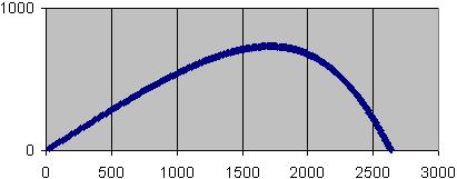
Finally, let us plot the trajectory of our projectile, accounting for the drag of a uniform atmosphere:
Note that the trajectory departs significantly from the parabola predicted when drag is not accounted for.
This method of separating the horizontal and vertical components has its limits. If we simulate firing a very light-weight object out of a gun at very high velocity and at a very low angle, our simulation fails. Under such circumstances, the trajectory curves upwards as the very high horizontal drag acceleration dominates the simulated motion. Obviously, this is non-physical behavior; drag force is always opposite the direction of motion and could not cause such a trajectory.