Rocket science and orbit simulation for hobbyists: Falling bodies and projectiles: using a more detailed atmospheric model

Falling Bodies and Projectiles

Part III: Using a More Detailed Atmospheric Model

This page originally compiled Mar 2007 by TFR

An interesting exercise, now that we have established a reasonably good model of the entire atmosphere, is to simulate the dropping of an object from outside that atmosphere, and to follow its trajectory to the ground. This is somewhat similar to the problem of simulating the reentry of an orbiting satellite, except that our object will drop straight down. We simulate here the same baseball which we have been dropping throughout these exercises. Once again, our baseball has a mass of 0.142 kg, a cross-sectional area of 0.00419 m², and a static C_d of 0.3. We simulate with a time step of 1 second, with the following results:
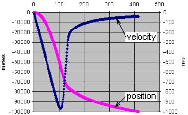picture: plot of velocity and altitude vs time of a baseball dropped from 100 km

picture: plot of velocity and altitude vs time of a baseball dropped from 100 km

Note that the baseball is virtually in unimpeded free fall until about 100 seconds from release, reaching a velocity of about 1 km/sec! At that point, about 50 km altitude, it begins to decelerate quite rapidly. As it enters the dense lower atmosphere, it approaches its typical terminal velocity as we have previously calculated. The baseball hits the ground after about 6 ¹/₂ minutes, giving us a rough upper limit for how long we could expect an object to fall within the atmosphere. This simulation is relatively coarse with a time step of 1 second, however its object is to show what can be accomplished with this type of simulation, rather than to give us accuracy. We reproduce here the first 10 seconds of the simulation as an example; see previous pages for explanation:

  density Mach #  Cd      acceler  init vel  final vel avg vel   position   time
  0.00000 0.00000 0.30030 -9.81000   0.00000  -9.81000  -4.90500   -4.90500  1
  0.00000 0.03399 0.30080 -9.81000  -9.81000 -19.62000 -14.71500  -19.62000  2
  0.00000 0.06800 0.30137 -9.81000 -19.62000 -29.43000 -24.52500  -44.14500  3
  0.00000 0.10204 0.30204 -9.81000 -29.43000 -39.23999 -34.33500  -78.47999  4
  0.00000 0.13611 0.30286 -9.80999 -39.23999 -49.04998 -44.14499 -122.62498  5
  0.00000 0.17024 0.30387 -9.80999 -49.04998 -58.85997 -53.95498 -176.57996  6
  0.00000 0.20444 0.30514 -9.80998 -58.85997 -68.66995 -63.76496 -240.34492  7
  0.00000 0.23872 0.30675 -9.80997 -68.66995 -78.47993 -73.57494 -313.91986  8
  0.00000 0.27308 0.30880 -9.80997 -78.47993 -88.28989 -83.38491 -397.30477  9
  0.00000 0.30756 0.31142 -9.80996 -88.28989 -98.09985 -93.19487 -490.49964 10

At each time step we calculate the density of the amosphere at this altitude, Mach number at current velocity and resulting C_d, and use these in the acceleration equation. Density, during the first 10 seconds, remains minute, appearing here as 0 to five decimal places, however Mach number and C_d begin to vary immediately.

picture: plot of falling velocity of a baseball, accounting for Mach number vs not accounting Let us now re-compute this simulation ignoring the effects of Mach number. Plotting a close-up section of the previous plot, we see that the velocities do not differ greatly except at the transition across the Mach 1 region, near 300 meters/second, amounting to about 20 seconds of elapsed time. We could conclude that for this particular object, a baseball, the additional burden of calculating the Mach number and its effect on drag may not be worth the trouble for a simplified simulation. Certainly, some objects probably exist where this would not be the case. For instance, if the particular terminal velocity happened to be near Mach 1, the object would spend considerable time there, and its trajectory would be significantly affected.

We now apply our model of the atmosphere to the problem of calculating drag on a projectile moving through it. We have previously found expressions for numerically evaluating the horizontal and vertical motion of an object, subject to gravity and to the drag of the air:
a = -g - (C_dρAv²) / (2m), for vertical motion
picture: plot of trajectory of projectile launched at 1500 m/s; uniform atmosphere vs standard atmosphere As before, in use of this equation we must take care of the sign of the drag term, that it be opposite the direction of motion.
a = (C_dρAv²) / (2m), for horizontal motion

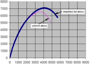
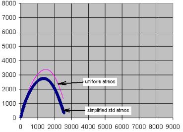
Previously, we assumed a uniform atmosphere under all circumstances of altitude and velocity. We now may substitute our calculated values of C_d and ρ at each time step of our simulation. Numerically simulating a projectile of frontal area A = 0.0002 m², mass m = 0.08 kg, coefficient of drag C_d0 = 0.2, using a time step of 0.1 second, we get the plotted results.
Above, our projectile has been launched at an angle of 80°, at 1500 m/s. Below, at 500 m/s. Note that at lower altitudes the increased drag of transition through Mach 1 causes the trajectory to undershoot the uniform atmosphere trajectory. At higher altitudes this effect is overcome and the reduced drag of the thinner atmosphere allows the trajectory to overshoot that of the uniform atmosphere, which does not diminish with altitude.
picture: plot of trajectory of projectile launched at 500 m/s; uniform atmosphere vs standard atmosphere This is one reason why most satellite-launching rockets are launched vertically and pitch over in the direction of the orbit only rather slowly. Lofting the vehicle above the lower atmosphere as rapidly as possible allows more efficient use of the limited fuel by avoiding the heavy drag of the denser air.

Home

Last Revised: Apr 2007