Chris R. Brown's physics and astronomy stuff
Radio Interferometer Simulator
Chris R. Brown's physics and astronomy stuff Radio Interferometer Simulator |
|||||
|
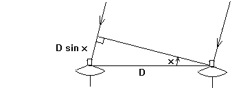
Simulation of a Meridian Transit Radio Interferometer Chris R. Brown, March 15, 1997 A diagram showing the geometry of a radio interferometer with two parabolic dishes is shown in Figure 1. The antennas could be yagis or horns. The preferred type of antenna depends on wavelength. Generally, energy from a distant source arrives at two antennas separated by a distance D.
As the earth rotates and the angle x slowly changes, the two antennas generate signals which are combined electrically.
This produces maxima and minima (called fringes by analogy with optical phenomena) as their phase relation changes. When
recorded, the fringe pattern is termed an interferogram. When many interferograms of the same radio source are collected, each for a different value of D, the distinctness of the
fringes, or "fringe visibility", varies. The details of this variation depend on the nature of the radio source. It is possible to extract information from this fringe visibility pattern, and learn the brightness distribution of the
radio source - that is, to get an image of an object in the sky in the light of radio waves. With this process
it is possible to convert our eyes from being sensitive to light to being sensitive to radio waves. This write up is
about simulating the first step in this process, getting interferograms. 1. Deriving a function to simulate an interferogram: The first thing to notice from Figure 1. is that
D sin x = n l ,
(1) where lambda is the center wavelength tuned by the antennas and electronics, and n is a real number. The variable n has
integer values when the two signals are exactly in phase, but n can have any value, and the two signals can be thought of
as sliding continuously in and out of phase as x changes with the earth's rotation. An easy way to represent the fringes is to say that as n varies between 0 and 1, (or between 1 and 2, etc.) one full fringe
cycle is seen. So we can make fringes with a function like
y = 1+ cos ( 2 p n
) .
(2) The use of the cosine function rather than the sine function is a way of saying the two signals will be in phase, and produce
a maximum, when n = 0, 1 ,2, etc. Equation (2) can be rewritten to bring in the measurable variables by solving eqn. (1) for n and substituting, to get y = 1 + cos ( 2 p ( D sin x / l ) ) . (3) The directivity pattern of the antenna L(x) can be approximately simulated with an exponential function of the form L(x) = exp
(- k ( x cos d )^2
/w ^2 )
(4) where k is a constant and w is the half-power beamwidth of the directivity pattern. The use of
the w ^
2 factor in the exponent provides linearity of beamwidth with the parameter w.
d is the declination
of the radio source, and the value of k is 2.7726 if a square law detector is assumed. Fringe visibility depends on D and on the angular extent of the radio source being observed, and is defined as V = ( Smax - Smin ) / ( Smax + Smin )
(5) and can be included in eqn 3. together with the directivity pattern L(x) by writing Y = Yzero L(x) [ 1 + V cos ( 2 p ( D sin x / l ) ) ] . (6) The factor Yzero is for scaling. The units of Y are proportional to radio brightness or power.
An offset term could also be added to eqn. 6 but is not shown in this development. The effect of the declination d also effects the rate of fringe production.
For a source away from the equator, fringes produced by an interferometer evolve more slowly than they would at the equator,
for the same antenna separation D ) the factor being simply cos d. So the final form of the equation describing fringe production is Y = Yzero L(x) [ 1 + V cos ( 2 p ( D sin x / l ) cos d ) ] . (7) Here is a personal note. When I first started thinking about this subject in 1995, there were many false starts and scribbling
numbers in margins and so forth. After a while, I got a good sense of how to think clearly about how a radio interferometer
works, and what I have written here is a result of that winnowing process. But this presentation doesn't reflect any of the
real process of discovery that is the most enjoyable part of working through a topic. After you read this, try forgetting
it and then start from scratch with a blank sheet of paper. When you get done, you'll have a good understanding too! 2. A computer program to simulate fringe production A computer program to do interferometer simulations is fairly easy to write and run. The process of writing such a program
helps develop and confirm the basic equations given in the preceeding section. Below is just such a program, written in QBASIC,
which comes with MS-DOS versions 5 and 6. For crying out loud, don't manually copy this program, contact me
directly and I'll e-mail the file to you. ' Simulated Solar Radio Interferometer Output' ' Chris R. Brown, Mar 22, 1997 ' Variable definitions: ' Lambda = wavelength in meters ' D = interferometer antenna spacing, meters ' Vis = fringe visibility, calculated from a function ' Lobe = a function that simulates the directivity of the antenna ' B = the primary antenna lobe beamwidth at half power, in degrees ' Ampl = an amplitude scaling factor ' NoiseAmp = peak amplitude of random noise ' Diam = assumed angular diameter of radio source, in degrees ' Dec = declination of radio source, in degrees ' SLambda = number of wavelengths between antennas ' Minutes = time in minutes, used as loop variable for earth rotation ' initialization: PI = 3.1416 Lambda = .075 '
Meters D =4 '
Meters SLambda = D / Lambda '
Number of wavelengths between antennas Diam = .5 '
Assumed radio source diameter, degrees Alpha = Diam / 57.3 '
Diam converted to radians B = 3.5 '
Half power antenna beamwidth in degrees W = B / 57.3 '
B converted to radians Dec = 17 '
Radio source declination, degrees DecRad = Dec / 57.3 '
Declination converted to radians Ampl = 1 NoiseAmp = .05
' Random noise added for realism ' Fringe visibility calculation: Vis = SIN(PI * SLambda * Alpha) / (PI * SLambda * Alpha) ' The program: PRINT INPUT " Enter DOS path and filename for data output > ", P$ PRINT OPEN P$ FOR OUTPUT AS #1 PRINT #1, PRINT #1, " Assumed radio source diameter in degrees = "; Diam PRINT #1, " Wavelength, Lambda, in meters = "; Lambda PRINT #1, " Antenna spacing, D, in meters = "; D PRINT #1, " No. of wavelengths between antennas, SLambda = "; SLambda PRINT #1, " Half power antenna beamwidth, in degrees = "; B PRINT #1, " Calculated fringe visibility, Vis = "; Vis PRINT #1, " Amplitude scaling factor, Ampl = "; Ampl PRINT #1, " Random noise peak amplitude, NoiseAmp = "; NoiseAmp PRINT #1, " Declination of radio source, in degrees = "; Dec PRINT #1, FOR Minutes = -30 TO 30 STEP .1 x = Minutes / 4 / 57.3 'converts Minutes to degrees to radians Lobe = EXP(-2.7726 * (x * COS(DecRad)) ^ 2 / W ^ 2) Noise = NoiseAmp * (RND - .5) fringe = (1 + Vis * COS((2 * PI * SLambda) * SIN(x) * COS(DecRad))) y = Ampl * Lobe * fringe + Noise WRITE #1, Minutes, y NEXT Minutes CLOSE #1 PRINT PRINT " The data is now in "; P$ PRINT END 3. Discussion of the interferogram simulator and its use To use the interferometer simulator and other related programs, first obtain the file TRANSIM.BAS by e-mail request
to me. Then start QBASIC ( in the DOS directory of MS DOS version 5.x or 6.x ) and load the radio interferometer
simulator file TRANSIM.BAS. You can run TRANSIM in a DOS shell, but some machines have issues with this practice.
I recommend using DOS. The first thing to notice about TRANSIM is that it is not a very big program. There is a section where parameter values
are defined, another section that writes these parameters to a disk file as a header, and then a dozen lines of code that
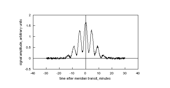
do the calculations and write the numeric results to the same file as the header. When TRANSIM is run, the output of the simulated interferometer is sent to a disk file as comma-delimited pairs. The
first number of each pair is the time after meridian transit in minutes, and the second is the simulated interferometer output,
in arbitrary units proportional to radio brightness. The best way to view the output is with a program that will draw graphs.
Excel will do this, and there are many others as well. As it comes out of the ZIP file, TRANSIM is programmed to output a number every 6 seconds for an hour. This results in
600 data points. You can change this and other parameters depending on what you want to simulate. You can see by looking at
the initialization section of TRANSIM that I used a central frequency of 4 GHz (7.5 cm) and a separation D
of 4 meters. The sun's declination was +17 degrees. A half-power beamwidth of 3.5 degrees was used to simulate an interferogram
that closely matches real data obtained with these same operating conditions. TRANSIM was run with
these parameters and the results are shown in figure 2.
|
||||||||